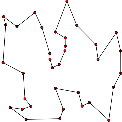
Given a graph $\graph$, compute the shortest tour linking all nodes.

$$ \begin{align} \min && \sum_{i, j \in E} x_{i,j} & \cdot \cost_{i,j} \\ s.t. && \sum_{j \in C} x_{i,j} & = 1 & \forall i \in C \\ && \sum_{j \in C} x_{j,i} & = 1 & \forall i \in C \\ && \sum_{i, j \in S} x_{i,j} & \leq |S| - 1 & \forall S \subseteq C \\ && x \in \B \end{align} $$

Given a graph $\graph$, a set of customer demands, and a set of identical vehicles $V$, compute the shortest routing so that all customers are visited once.

$$ \begin{align} \min && \sum_{v \in V} \sum_{i,j \in E} & x_{i,j}^v \cdot \cost_{i,j} \\ s.t. && \sum_{v \in V} y^v_i & = 1 & \forall i \in C \\ && \sum_{i \in C} y^v_i \cdot \dem_i & \leq \capa & \forall v \in V \\ && y^v_i & \leq \sum_{j \in C} x_{j,i}^v & \forall v \in V, i \in C \\ && \sum_{j \in C} (x_{j, i}^v - x_{i, j}^v) & = 0 & \forall v \in V \\ && \sum_{i, j \in S} x^v_{i,j} & \leq |S| - 1 & \forall S \subseteq C, v \in V \\ && x \in \mathbb{B}&, y \in \mathbb{B} \end{align} $$

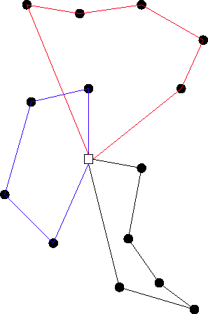
Relaxation of the VRP where customers can be visited more than once.

• Based on a tender to optimise grocery delivery in Queensland
• First MIP model developed in [1] as a benchmark for comparison against CP
• Can be extended using valid cuts or symmetry breaking
• Fleet and routing can be modelled in numerous ways
  • Composite model

• Gurobi v6.5
• 15min runs
• Based on real data
• Three category of instances: small, medium, large